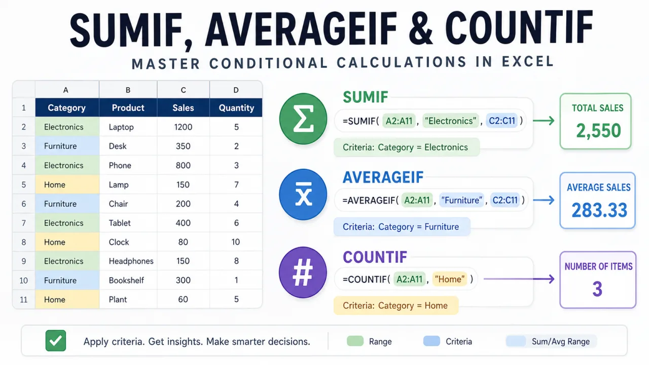
SUMIF, AVERAGEIF, and COUNTIF answer three different questions from the same type of condition. SUMIF asks, "What is the total where this condition is true?" AVERAGEIF asks, "What is the average where this condition is true?" COUNTIF asks, "How many cells match this condition?" Once you understand the shared structure, the formulas become much easier to remember because the criteria logic is almost identical.
The key is to separate the criteria range from the calculation range. The criteria range is the column Excel checks. The calculation range is the column Excel adds or averages. COUNTIF does not need a calculation range because it is counting the matching cells themselves. This small difference explains most of the confusion people run into when moving between the three formulas.
SUMIF syntax and usage
The basic syntax is =SUMIF(range, criteria, sum_range). The range is where Excel looks for the condition. The criteria is what Excel tries to match. The sum_range is what Excel adds when the condition is true. If products are in A2:A20 and sales are in C2:C20, the total sales for Laptop is =SUMIF(A2:A20,"Laptop",C2:C20).
Use SUMIF when you want one condition. Typical examples include total revenue for one region, total expenses for one category, total units for one sales rep, or total profit for one product line. If you need two or more conditions, use SUMIFS. The order changes slightly in SUMIFS: the sum range comes first, then each criteria range and criteria pair follows.
AVERAGEIF syntax and usage
The syntax is =AVERAGEIF(range, criteria, average_range). It behaves like SUMIF, but it divides the matching total by the number of matching values. If regions are in B2:B20 and sales are in C2:C20, the average sale for East is =AVERAGEIF(B2:B20,"East",C2:C20). This is helpful when the total alone would be misleading. A region with more orders may have higher total revenue, but a lower average deal size.
Blank cells in the average range are ignored. Zeroes are not ignored. That matters when analyzing performance. A blank may mean no recorded value, while a zero may mean a real zero sale. Before using AVERAGEIF, decide whether blank values and zero values mean the same thing in your sheet. If they do not, clean the data or add a second condition with AVERAGEIFS.
COUNTIF syntax and usage
The syntax is =COUNTIF(range, criteria). There is no separate count range because Excel counts cells in the criteria range that match the condition. If product names are in A2:A20, use =COUNTIF(A2:A20,"Laptop") to count how many rows contain Laptop. If you need a row-by-row duplicate number instead of a final count, use the expanding range approach explained in running count of occurrence in Excel.
Criteria examples that work in all three formulas
Criteria can be exact text, a number, a comparison, a wildcard, or a cell reference. For exact text, place the text in quotation marks, such as "Laptop". For comparisons, place the operator and number in quotation marks, such as ">500". To compare against a cell, join the operator to the cell reference with &, such as ">"&F2. Wildcards are useful for partial matching. "East*" matches values that begin with East. "*Pro*" matches any value containing Pro.
| Question | Formula | Notes |
|---|---|---|
| Total sales for East | =SUMIF(B2:B20,"East",C2:C20) | Checks region, adds sales. |
| Average sales above 500 | =AVERAGEIF(C2:C20,">500",C2:C20) | The same range can be used for criteria and average. |
| Count products containing Pro | =COUNTIF(A2:A20,"*Pro*") | The asterisks mean any characters before or after Pro. |
| Total for category in F2 | =SUMIF(A2:A20,F2,C2:C20) | Use a cell reference to make the report reusable. |
Common mistakes
The first mistake is using ranges of different sizes. =SUMIF(A2:A20,"Laptop",C2:C500) is a warning sign because the criteria range and sum range do not line up. Keep the ranges the same height. The second mistake is putting the criteria in the wrong range. If you are checking product names, the criteria range must be the product column, not the sales column. The third mistake is forgetting quotation marks around operators. >500 alone is not valid criteria. Use ">500".
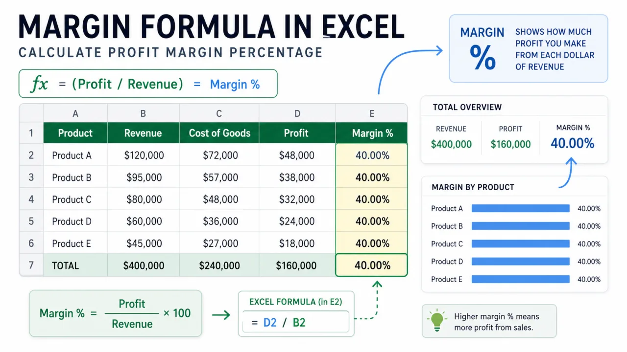
Another mistake is trying to use SUMIF for profit margin. SUMIF can total revenue and cost by category, but a margin percentage still needs the relationship between profit and revenue. If that is the metric you need, the margin formula in Excel guide shows the safer way to build the percentage after the totals are calculated.
When one condition is not enough
The single-condition formulas are best when the question has one filter. Total sales for Laptop is a one-condition question. Average revenue for East is also one condition. As soon as the question says "Laptop in East" or "orders above 500 in June", move to the plural versions: SUMIFS, AVERAGEIFS, and COUNTIFS. The plural formulas let you pair each criteria range with its own condition, which keeps the workbook clearer than trying to combine several checks in helper columns.
There is one important syntax shift. In SUMIF, the sum range is last. In SUMIFS, the sum range is first. For example, =SUMIFS(C2:C20,A2:A20,"Laptop",B2:B20,"East") adds sales from C2:C20 only where the product is Laptop and the region is East. The average and count versions follow the same idea. Once you get used to reading the formula as "calculate this range where these conditions are true", the order becomes easier to remember.
A good workflow is to write the formula against a small visible section first, manually check two or three matching rows, then expand the formula into the full report. If you are building a summary area, put the criteria in cells and reference those cells rather than rewriting text criteria inside every formula. That makes the sheet easier to update and reduces spelling mistakes. These formulas are simple, but they become powerful when the ranges are clean, the criteria are visible, and the result is checked against the raw data.