Writing a month as a number in Excel sounds simple until the source data changes shape. One column may contain real dates such as 6/11/2026. Another may contain month names such as June. Another may contain abbreviated text such as Jun. Excel handles those cases differently. The right method depends on whether the cell is a real date value, text that looks like a month, or a messy import that needs cleanup before it can be used in formulas, pivots, charts, or dashboards.
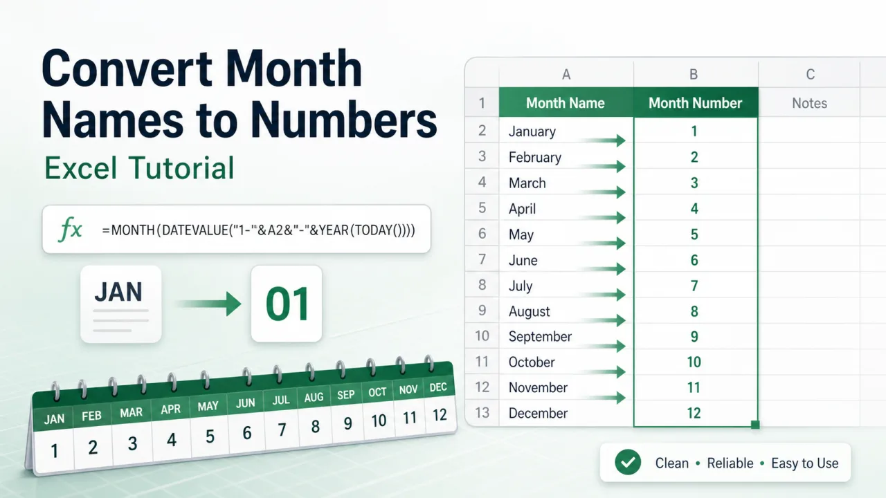
If the cell contains a real Excel date, use =MONTH(A2). That returns a number from 1 to 12. January returns 1, February returns 2, and December returns 12. This is the most reliable method because Excel already understands the date. If the cell contains only text such as January, use =MONTH(DATEVALUE(A2&" 1")). The added " 1" gives Excel a day number so the month name can be interpreted as a date.
When the source cell is a real date
The easiest case is a true date. If A2 contains 6/11/2026, type =MONTH(A2). The result is 6. This works because Excel stores dates as serial numbers behind the scenes. The date format you see on screen is only formatting. The underlying value is still a date number, so MONTH can read it directly.
If you only want the month number to display as two digits, use formatting or the TEXT function. =TEXT(A2,"mm") returns 06 as text. This is useful for labels, filenames, or codes where leading zeroes matter. If you need to sort or calculate, keep the numeric result from =MONTH(A2). If you need a display label, use TEXT.
When the source cell is a month name
If A2 contains June, Excel may not treat it as a date. =MONTH(A2) can fail because there is no day or year attached. The safer formula is =MONTH(DATEVALUE(A2&" 1")). If A2 is June, the expression creates June 1, DATEVALUE turns that into a date, and MONTH returns 6.
This approach also works with many abbreviated month names such as Jan, Feb, and Sep, depending on the language settings of the workbook. If your workbook receives data from different countries, avoid relying only on text recognition. A small lookup table is more predictable because it maps each accepted spelling to the number you want.
Use a lookup table for controlled month names
A lookup table is the best method when the source data is inconsistent. Put accepted month names in one column and the correct number in the next column. Then use a lookup formula. For example, if your lookup table is in F2:G13, use =XLOOKUP(TRIM(A2),F2:F13,G2:G13). The TRIM function removes accidental spaces. You can include versions such as Jan, January, Sept, and September if your files use mixed naming.
A lookup table is less elegant than a single MONTH formula, but it is easier to audit. A manager can look at the mapping and confirm that each spelling is handled correctly. It also avoids regional date interpretation problems. For example, a text date like 03/04/2026 can mean March 4 or April 3 depending on settings. A controlled month mapping removes that ambiguity.
| Input type | Recommended formula | Result type |
|---|---|---|
| Real date in A2 | =MONTH(A2) | Number from 1 to 12 |
| Real date, two digit display | =TEXT(A2,"mm") | Text such as 06 |
| Month name in A2 | =MONTH(DATEVALUE(A2&" 1")) | Number from 1 to 12 |
| Messy imported name | =XLOOKUP(TRIM(A2),F2:F13,G2:G13) | Controlled mapped number |
Build a year month key
Month numbers are often used for sorting. If you sort by month name, April can come before February because text sorts alphabetically. If you sort by month number alone, January 2025 and January 2026 group together even if they belong in different years. A better reporting key is year plus month. If A2 contains a real date, use =TEXT(A2,"yyyy-mm"). It creates sortable labels such as 2026-01, 2026-02, and 2026-12.
Keep calculation numbers separate from display labels
One practical mistake is using a text month code where a number is needed. =TEXT(A2,"mm") returns a text value that looks like a number. That is fine for labels, but it can create confusion if another formula expects a numeric month. If you need to compare months with >, sort them as numbers, or use them in arithmetic, use =MONTH(A2). If you need a pretty label for a file name, dashboard header, or export code, use TEXT.
A clean workbook can keep both fields. One column can hold the numeric month from MONTH. Another column can hold the display month from TEXT. The numeric field drives sorting, filters, and formulas. The display field appears in reports. This avoids the common problem where a sheet looks correct on screen but sorts or calculates incorrectly because the visible number is actually text.
If your next step is a chart, take time to choose the right month output. A numeric month is good for grouping within one year. A year month key is better for a timeline. Clean month numbers also help when you later build a standard deviation graph in Excel, because chart order and clean labels matter as much as the formulas behind the chart.
Quick checks before using the month number
Before using the converted month in a report, filter the result column and scan the unique values. A proper month number column should contain only 1 through 12. If you see blanks, errors, or unexpected text, the source data needs attention. Check for trailing spaces, invalid month names, mixed languages, and dates imported as text. A short check at this stage prevents broken pivot tables and charts later.
If the month column is used by other people, add a short header note such as "numeric month for sorting" or "display month only." That makes the intent clear. Month conversion is not a difficult Excel task, but the workbook becomes much more reliable when the number used for calculation is separated from the label used for presentation.